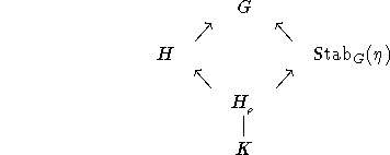
Generating diagrams is relatively straightforward. Think of the
diagram as a 2-dimensional array, with
each entry filled by a symbol or a blank.
These ``arrays'' are defined in  as in the following example:
$$\begin{array}{rcccl}
           \; & \; & G      &\;       &\; \\
           \; & \nearrow      & \; & \nwarrow  &\; \\
           H      & \; & \; & \;      &\text{Stab}_G(\eta) \\
           \; & \nwarrow & \; & \nearrow       &\; \\
           \; & \; & H_{_\rho}   & \;  &\; \\
           \; & \; & \mid   &\;       &\; \\
           \; & \; & K      &\;       &\;
\end{array}$$
The argument {rcccl} works the same way as the argument
to the tabular environment, described in
Section 6.7.
Here, {rcccl} specifies that there are 5 columns, of which the
first is right-justified, the middle four centered, and the last
left-justified.
As in the tabular environment,
each row ends with a carriage return \\, and ampersands
& separate entries in
a given row.
Since we are making a diagram,
some entries are arrows, others symbols, and many
blank.
The command sequence above generates
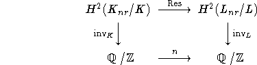
![]() includes the same automatic generator of rectangular commutative
diagrams contained in A
MS-
includes the same automatic generator of rectangular commutative
diagrams contained in A
MS-![]() when you load the
when you load the amscd package.
You can then type
\begin{CD}
H^2(K_{nr}/K)   @>{\operatorname{Res}}>>   H^2(L_{nr}/L)\\
@V{\operatorname{inv}_K}VV      @VV{\operatorname{inv}_L}V \\
{\mathbb Q}/{\mathbb Z}    @>n>> {\mathbb Q}/{\mathbb Z}
\end{CD}
to make the diagram
Read the next section to learn how to avoid typing \operatorname
all the time ![]() .
.