In Unix, you start matlab by typing "matlab"
at the command line. If you don't want
to start matlab with a user interface, type
matlab -nodesktop -nosplash
You quit it with "exit;". You can also put the commands into a file
"script.m" and enter
matlab < script.m > script.out &
A good starting point is to type "demo" within matlab.
Besides programming, matlab can be used as a powerful
"calculator". For example, in linear algebra, you
would evalute the determinant,
the inverse, characteristic polynomials or eigenvalues of a matrix:
a = [1 2 3; 4 5 6; 2 3 7]; det(a)
inv(a)
poly(a)
eig(a)
For calculus, you might want to integrate symbolically
int(1/(1+x^2))
or numerically
quad('sin(x)-x',0,pi)
or differentiate
diff('tan(x)*x')
You can plot functions of one variables
 fplot('sin',[0,10])

 t=0:0.1:10; y=sin(t); plot(t,y)
or two variables
[x,y]=meshgrid(-1:.2:1,-1:.2:1); z=exp(-x.^2+y.^2); mesh(z)
|
visualize data (for example matrix entries):
a=rand(100); b=inv(a); imagesc(b);
a=magic(100); imagesc(a);
find the roots of polynomials for example of
p(x)=9x5+2x4+3x3+4x2+5x+7:
roots([9 2 3 4 5 7])
or finding the next root more general functions starting near a point
fzero('cos(x)-x',0.5)
visualize graphs (like for example the Buckminster Fuller geodesic dome):
[B,V]=bucky; gplot(B,V);
doing polynomial fits:
x=(0:0.1:5)'; y=sin(x); p=polyfit(x,y,1); f=polyval(p,x); plot(x,y,'o',x,f,'-');
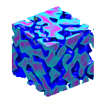
It even has rendering capabilities:
data = rand(12,12,12);
isoval = .4;
h = patch(isosurface(data,isoval),...
    'FaceColor','blue',...
    'EdgeColor','none',...
    'AmbientStrength',.2,...
    'SpecularStrength',.7,...
    'DiffuseStrength',.4);
isonormals(data,h)
patch(isocaps(data,isoval),...
    'FaceColor','interp',...
    'EdgeColor','none')
colordef black;
colormap cool;
daspect([1,1,1]);
axis off; view(3);
camlight right;
camlight left;
set(gcf,'Renderer','zbuffer');
material shiny;
lighting phong;
These few lines have produced the graphics near the title.
|

